How to Enhance Algo Trading Win Rate with ML: Training

Previously on "How to Enhance Algo Trading Win Rate with ML":

If you want to maximize the performance of developing and coding, please read "How to Enhance Algo Trading Win Rate with ML: Labelling Data" and “How to Enhance Algo Trading Win Rate with ML: Feature Selection” before proceeding.

In the first article, we discussed data labeling through the SMA crossover strategy and the manual correction of labels to enhance the quality of the input data for our machine-learning model.

In the second article, we examined the diversity and reliability of our features and compared them to select the best possible features for our training phase.

In this article, we intend to experimentally train the features we have selected using the TensorFlow and Keras libraries.

 

Part 3: Training

TensorFlow and Keras are both powerful libraries used in machine learning and deep learning.

TensorFlow is an open-source machine learning framework developed by Google. It is designed to facilitate the development of large-scale machine-learning models and make them available for deployment on a wide range of platforms. TensorFlow provides an extensive set of tools for building and training machine learning models, including support for building deep neural networks.

Keras is a high-level neural network API that runs on top of TensorFlow. It provides an easy-to-use interface for building and training deep learning models. Keras is widely used in the machine learning community due to its simplicity, flexibility, and ease of use. With Keras, you can quickly build complex neural network architectures and train them on large datasets.

Together, TensorFlow and Keras provide a powerful platform for developing and training machine learning models. In this article, we explain how to use Keras to build and train a deep learning model, leveraging the features provided by TensorFlow to optimize performance and scalability.

Our experiment will be implemented in the "Jupyterlab" environment. Clone the improve_algorithmic_trading_ml repository and run the 3-train_long.ipynb and 3-train_short.ipynb for a better understanding.  We divided the entire dataset into long and short segments during training to enable us to optimize the model's features and parameters according to the unique characteristics and size of each segment, resulting in improved performance.

Together, we will undergo training for the long model, and then you can apply the same approach to the short model.

 

Block [1-3]

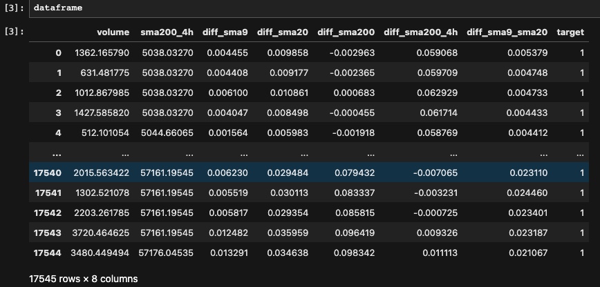
To begin with the training process, we will import the dataset that was constructed during the feature selection phase and eliminate any unnecessary columns from it in order to make it ready for training.

 

Block[4-7]

We need to preprocess data for training a machine learning model in TensorFlow using feature columns to make it easier to train a neural network and improve the accuracy of the resulting model.

To achieve that we start by splitting the dataframe into training, validation, and testing sets using the train_test_split function from the scikit-learn library.

Then, we define the df_to_dataset function, which takes our dataframe and converts it into a TensorFlow dataset. The function shuffles the data, removes the 'target' column, and stores it separately as the labels. It also returns the dataset with the specified batch size which in our case is 32. We apply this function to create the train, validation, and test datasets with a batch size of 32. The validation and testing datasets are not shuffled since we don't need to randomize the order of examples for these datasets.

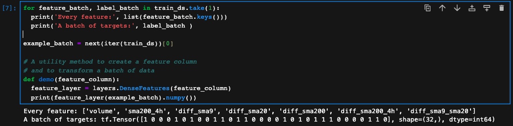
And finally, we define a utility function called demo, which takes a feature column as input, creates a DenseFeatures layer using the feature column, and transforms a batch of data using the layer. The DenseFeatures layer is used to transform the raw input data into a dense tensor that can be fed into the neural network. While it is not obligatory to define and utilize this function in our training, doing so provides us with a comprehensive understanding of how the feature layer operates in TensorFlow.

 

Block[8-11]

Now that we have prepared all our datasets, the next step is to choose the relevant features and provide them for training. We will begin by processing the features identified during the previous phase to understand their individual characteristics, based on the experiments conducted. Additionally, we will incorporate a mix of experiments by adding or removing certain features during training to evaluate the outcomes. In TensorFlow, there are various feature types available, and you can refer to the official documentation to learn how to utilize them effectively. For our purposes, we will specifically utilize two feature types: numeric column and bucketized column.

• Numeric Column: This feature column is used for representing numerical features. It accepts numeric data and performs no additional transformations on the input.
• Bucketized Column: This feature column is used for discretizing numeric features into buckets or bins. It takes a NumericColumn as input and divides the values into specified buckets

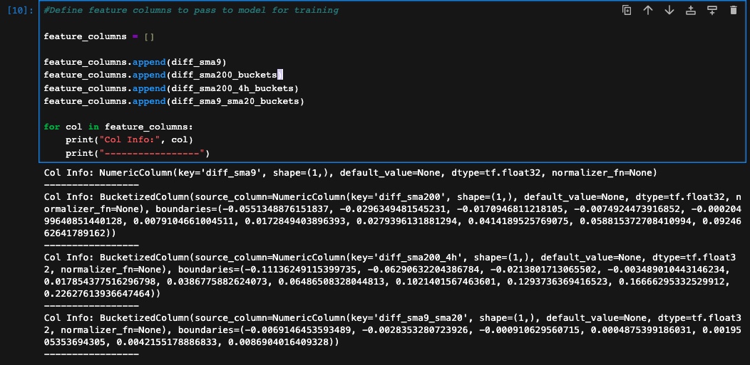
We also keep the bucketized column boundaries in a separate file so that we can bucketize the columns with the same bounds for future use. We then create the feature layer with the bucketized and numeric columns. A feature layer in TensorFlow Keras is an input layer that simplifies the preprocessing of input features for a neural network model. It encapsulates operations like normalization, one-hot encoding, and feature transformations within the layer. This allows for consistent and reusable preprocessing steps across training and inference. Feature layers enable easy organization and combination of different feature types, making it simpler to construct complex models with multiple input branches.

 

Block [12-15]

As mentioned before we use the Keras library in our experiment for training. Keras uses various methods for training deep neural network models. The one we use is sequential. We will first define the model with its parameters and save it in a separate file.  By following this approach, we have the flexibility to modify and adapt it independently to incorporate various features as needed.

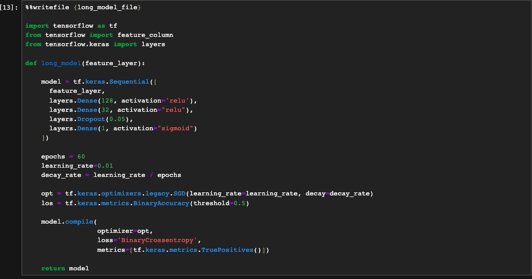
The long_model function defines a sequential model, which means the layers are stacked linearly on top of each other. The model starts with a feature layer, which is a placeholder for input features.

Following the feature layer, there are three fully connected (dense) layers defined with different sizes: 128 units with ReLU activation, 32 units with ReLU activation, and 1 unit with sigmoid activation. The ReLU activation function introduces non-linearity into the model, while the sigmoid activation function is suitable for binary classification tasks as it outputs a probability between 0 and 1.

The model also includes a dropout layer with a rate of 0.05, which helps prevent overfitting by randomly disabling a fraction of the units during training. This encourages the model to learn more robust representations.

After defining the model architecture, we specify the number of epochs (60 in this case) and the learning rate. The learning rate is used to control the step size during model optimization. Additionally, a decay rate is calculated based on the learning rate and the number of epochs to gradually reduce the learning rate over time.

Then we create an optimizer using stochastic gradient descent (SGD) with the specified learning rate and decay rate. The loss function is set to binary cross-entropy, which is commonly used for binary classification tasks. The model's performance is evaluated using the binary accuracy metric and the number of true positives.

Finally defining all of that parameters for our model we can use the model to train our data.

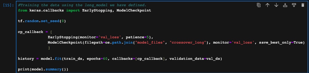
In the above cell, we first import two classes from the Keras callbacks module: EarlyStopping and ModelCheckpoint. These classes provide functionalities that help us monitor the training process and save the best version of our model.

Next, we set a random seed using the TensorFlow library to ensure the reproducibility of the results. This means that if we run the code multiple times, we will get the same random numbers generated.

Then, we create a list called cp_callback, which will hold our callback objects. Callbacks are special functions or objects that can be called during the training process to perform specific actions. In this case, we have two callbacks in the list:

• EarlyStopping: This callback monitors the validation loss during training and stops the training process early if the loss doesn't improve for a certain number of epochs. The monitor=val_loss parameter specifies that we are monitoring the validation loss, and the patience=5 parameter means that if the validation loss doesn't improve for 5 consecutive epochs, the training will stop.
• ModelCheckpoint: This callback saves the best version of the model based on the validation loss. The filepath parameter specifies the path and filename where the best model will be saved. The monitor=val_loss parameter tells the callback to consider the validation loss when deciding which model is the best, and the save_best_only=True parameter ensures that only the best model is saved.

After setting up the callbacks, we can train our model. The model.fit() function is used to train our machine learning model.

 

Block [16-18]

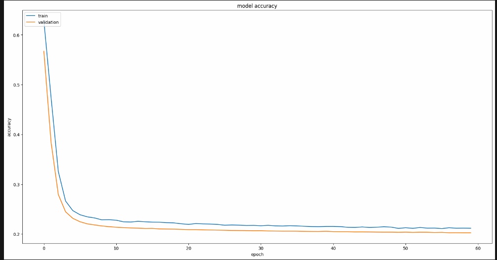
Now that the training is done we examine the model's accuracy and how it evolves over the training process. By visualizing the training and validation losses, we gain insights into how well the model is learning. By comparing the trends of the training and validation losses, we can assess whether the model is overfitting or underfitting. If the validation loss follows a similar trend to the training loss, it suggests that the model is generalizing well. The resulting plot helps us understand the progress of the training and visualize any potential issues.

In the second part, we evaluate the model's accuracy on a separate test dataset. By using the model.evaluate() function, we obtain the loss and accuracy metrics of the model on the test data. This information provides an objective measure of the model's performance.

Lastly, by using the model.save_weights() function, we can store the learned parameters of the model, including the weights and biases, in a specified file location. This step ensures that we can easily reload the model in subsequent sessions without needing to retrain it from scratch.

 

Our long training phase has finished now and now we can go over the same flow for the short training. You can demonstrate that by modifying and running the 3-train_short.ipynb file.

Throughout this experiment, it is important to note that training a machine learning model requires iteratively adjusting features and model parameters to achieve desirable results. It's crucial to recognize that making modifications to the way we select and train our model can potentially enhance its accuracy. With this in mind, we have the opportunity to further refine our approach and attain even better results.

In the next article, we will leverage the knowledge gained from training our model to make predictions on new data. Additionally, we use the backtest strategy to evaluate whether our machine learning model has improved the win rate of our algorithmic trading.